The Hardness of Validating Observational Studies with Experimental Data

Introduction and motivation

Many models at Spotify are trained using randomized data to prevent bias. In many cases, the size of this randomized data is only a small fraction of all activity on Spotify. This can lead to generalizability issues, as well as sub-optimal impact in areas such as messaging and promotions—as we can’t optimize impact in the randomized data. One approach to address this issue is to supplement the randomized data with passively collected observational data. This increases the size and variation of the training dataset, which should increase generalizability, but this may come at a cost by introducing bias inherent in observational data. 

In addition to model training, there are many other uses to combining randomised data with observational data. Randomized controlled trials typically cannot be run for long periods of time, so combining with appropriate observational data can extend the findings from the trial to longer time periods. In the other direction, data from randomized trials can be used to falsify findings from the observational data, or to benchmark the amount of bias—or unmeasured confounding—in the observational data.

In our recent paper, we studied the general problem of combining randomized and observational data and have proved fundamental limitations to this approach, as well as what assumptions are needed to overcome them. We end by providing practical approaches to implement such assumptions in practice.

Formulating the problem

To formalize the problem, we introduce a function called the gap, denoted as Δ(x). This is defined as the difference between the Conditional Average Treatment Effect (CATE) estimated from randomized experimental data and that from observational data at a particular value of covariates, x:

Δ(x)=τ(x)−ω(x) 

Here, τ(x) is the true causal effect—identifiable under randomization—and ω(x) is the modelled effect from observational data. If Δ(x) is zero, our observational model is unbiased. But the more Δ(x) differs from zero, the more confounding (bias) exists in our observational estimate.

Hypothesis Testing Setup

We use the language of hypothesis testing to explore whether we can measure or bound this gap using experimental data. Specifically, we consider testing whether Δ(x) lies within a predefined range—like asking, “Is the bias small enough to be acceptable?”

Two types of hypothesis tests are defined:

• Falsification Tests: Can we reject the idea that bias is small? (i.e., is Δ(x) outside the acceptable range?)

• Validation Tests: Can we confirm that bias is small? (i.e., is Δ(x) inside the acceptable range?)

These questions are closely related to scientific falsification and equivalence testing in medicine, such as when testing whether a generic drug is “close enough” in effect to a branded one.

Main theoretical result: The tension between validation and falsification

While falsification tests are statistically feasible, our main theoretical results is to show that validation tests are fundamentally impossible without additional assumptions. In other words, we can use randomized data to witness if a model trained on observational data is wrong—but not to confirm that it's right. 

Using the framework of impossible inference from econometrics, we show that although it is possible to use experimental data to falsify causal effect estimates from observational data, in general it is not possible to validate such estimates. Our theorem proves that while experimental data can be used to detect bias in observational studies, without additional assumptions on the smoothness of the correction function, it can not be used to remove it. 

This is due to the fact that even if Δ(x) lies within a desired range in a dataset, there could always be other distributions with unmeasured spikes in bias that are statistically indistinguishable but fall outside this range. Therefore, no matter how much data we collect, we can’t confidently say the observational estimate is unbiased.

The main intuition behind the proof of our result is graphically illustrated in the below figure.

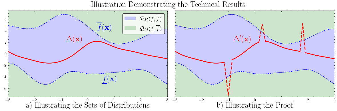
• The left panel shows two regions of distribution space: one where bias Δ(x) is always within bounds (blue region), and one where it isn’t.

• The right panel shows how, for any distribution inside the blue region, you can always construct a nearly identical one just outside of it, by adding “spikes” to Δ(x). These spikes are undetectable with finite data but violate the assumption of bounded bias.

This means there is no statistical test that can guarantee that Δ(x) lies within a safe zone—only that it sometimes doesn’t. More formally, our theorem showed that there are no verification hypothesis tests that can distinguish all alternatives from the null hypothesis, but there are falsification hypothesis tests that do.

Implications for Sensitivity Models

Sensitivity models are a common tool used to quantify the strength of potential unmeasured confounding. Our paper shows that we can only lower-bound the amount of confounding from data. That is, we can say, “there must be at least this much bias,” but not, “there is no more than this much bias.”

This has meaningful implications: you can't confirm that an observational causal effect estimate is robust to unmeasured confounding using experimental data—unless you make assumptions on the relation between the observational and experimental dataset.

Circumventing the Theorem with Smoothness Assumptions

The core difficulty arises because Δ(x) is allowed to be arbitrarily “spiky” (i.e., non-smooth). If we instead assume that Δ(x) is smooth—for example, that it comes from a Gaussian Process (GP)—we can circumvent the theorem and make meaningful inferences.

Gaussian Processes are flexible, probabilistic models that assume the function we’re trying to learn (in this case, Δ(x)) changes gradually. Under this assumption, our paper introduces a novel GP-based method that learns Δ(x) from pseudo-outcomes—transformed versions of the experimental data that allow learning without violating statistical assumptions.

The approach comes with uniform error bounds, ensuring that the predicted treatment effects are accurate across the entire observational support with high probability. This lets practitioners create confidence intervals that remain valid even outside the experimental data.

Final Thoughts

Our work highlights a critical nuance in causal inference: while combining observational and randomized data is intuitively appealing, it can’t address unmeasured confounding unless you’re willing to make assumptions—such as smoothness in the bias function. The proposed GP method shows a practical and principled way to do just that, offering both improved predictive performance and well-calibrated uncertainty.

By recognizing the limits of what can be statistically proven—and designing methods that work within those limits—our paper offers a realistic roadmap for using all available data in a principled way.

For more information, please refer to our paper: The hardness of validating observational studies with experimental data Jake Fawkes, Michael O’Riordan, Athanasios Vlontzos, Oriol Corcoll, Ciarán Gilligan-Lee AISTATS 2025