Survival Analysis Meets Reinforcement Learning

TL;DR: Survival analysis provides a framework to reason about time-to-event data; at Spotify, for example, we use it to understand and predict the way users might engage with Spotify in the future. In this work, we bring temporal-difference learning, a central idea in reinforcement learning, to survival analysis. We develop a new algorithm that trains a survival model from sequential data by leveraging a temporal consistency condition, and show that it outperforms direct regression on observed outcomes.
Survival analysis
Survival analysis is the branch of statistics that deals with time-to-event data, with applications across a wide range of domains. Survival models are used by physicians to understand patients’ health outcomes. Such models are also used by engineers to study the reliability of devices ranging from hard drives to vacuum cleaners. At Spotify, we use survival models to understand the way users will engage with Spotify at a later date.. Such models are important to ensure that Spotify makes decisions that are aligned with our users’ long-term satisfaction—from tiny decisions such as algorithmic recommendations all the way to big changes in the user interface.
Here is a typical scenario for survival analysis. Suppose that we are interested in predicting, for every Spotify user with a free account, the time until they convert to a Premium subscription. We call this conversion the “event”. To learn a model that predicts the time-to-event, we start by collecting a dataset of historical observations.
We select a sample of users that were active a few months ago, and obtain a feature vector that describes how they were using Spotify back then.
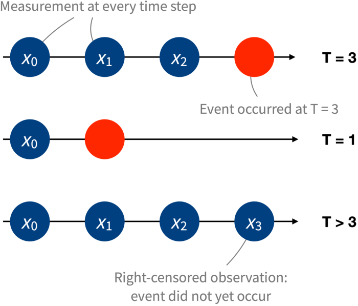
We then fast-forward to the present and check if they have converted in the meantime. For those users who converted, we record the time at which it happened. Note that many users in the sample will not yet have converted, and the technical term for these observations is “right-censored” (the time-to-event is above a given value, but we do not know by how much). These observations still carry useful signals about the time-to-event.
With this we have constructed a dataset of triplets (x0, t, c), one for each user in the sample. We call x0 the initial state; it describes the user at the beginning of the observation window (i.e., a few months ago). The second quantity, t, denotes the time-to-event (if the user has converted since the beginning of the window) or the time until the end of the observation window. Finally, c is a binary indicator variable that simply denotes whether the user has converted during the observation window (c = 0) or not (c = 1).
The next step is to posit a model for the data. One model that is very simple and popular is called the Cox proportional-hazards model. At Spotify, we have also had good results with Beta survival models. Given a dataset of observations, we can train a model by maximizing its likelihood under the data—a standard approach in statistics and machine learning. Once we have trained such a model, we can use it to make predictions about users outside of the training dataset. For example, a quantity of interest is

the probability that a user’s time-to-event T is larger than k, given the user’s initial state x0.
The dynamic setting
Increasingly, it is becoming commonplace to collect multiple measurements over time. That is, instead of only having access to some initial state x0, we can also obtain additional measurements x1, x2, … collected at regular intervals in time (say, every month). To continue with our example, we observe not just how long it takes until a free user converts but also how their usage evolves over time. In clinical applications, from an initial state indicating, for instance, features of a patient and a choice of medical treatment, we might observe not just the survival time but rich information on the evolution of their health.
In this dynamic setting, the data consist of sequences of states instead of a single, static vector of covariates. This naturally raises the question: Can we take advantage of sequential data to improve survival predictions?
One approach to doing so is called landmarking. The idea is that we can decompose sequences into multiple simpler observations. For example, a sequence that goes through states x0 and x1 and then reaches the event can be converted into two observations: one with initial state x0 and time-to-event t = 2, and another one with initial state x1 and time-to-event t = 1.
This is neat, but we suggest that we can do even better: we can take advantage of predictable dynamics in the sequences of states. For example, if we know very well what the time-to-event from x1 is like, we might gain a lot by considering how likely it is to transition from x0 to x1, instead of trying to learn about the time-to-event from x0 directly.
A detour: temporal-difference learning
In our journey to formalizing this idea, we take a little detour through reinforcement learning (RL). We consider the Markov reward process, a formalism frequently used in the RL literature. For our purposes, we can think of this process as generating sequences of states and rewards (real numbers): x0, r1, x1, r2, x2, … A key quantity of interest is the so-called value function, which represented the expected discounted sum of future rewards from a given state:

where γ is a discount factor. Given sequences of states and rewards, how do we estimate the value function? A natural approach is to use supervised learning to train a model on a dataset of empirical observations mapping a state x0 to the discounted return

In the RL literature, this is called the Monte Carlo method.
There is another approach to learning the value function. We start by taking advantage of the Markov property and rewrite the value function as

This is also called the Bellman equation. This suggests a different way to use supervised learning to learn a value function: instead of defining the regression target as the actual, observed discounted return, define it as the observed immediate reward r1, plus a prediction at the next state, γV(x1), where the value at x1 is given by a model. This might look like circular reasoning (using a model to learn a model!), but in fact this idea is central in reinforcement learning. It is known under the name of temporal-difference learning, and has been a key ingredient in the success of RL applications over the past 30 years.
Our proposal: temporally-consistent survival regression
We now return to our dynamic survival analysis setting, and to the problem of predicting time-to-event. Is there something we can learn from temporal-difference learning in Markov reward processes? On the one hand, there is no notion of reward, discount factor or value function in survival analysis, so at first sight it might look like we are dealing with something very different. On the other hand, we are also dealing with sequences of states, so maybe there are some similarities after all.
A crucial insight is the following. If we assume that the sequence of states x0, x1, … form a Markov chain, then we can rewrite the the survival probability as

for any k ≥ 1. Intuitively, this identity states that the survival probability at a given state should be similar (on average) to the survival probability at the next state, accounting for the delay. This looks very similar to the Bellman equation above. Indeed, in both cases, we take advantage of a notion of temporal consistency to write a quantity of interest (the value function or the survival probability) recursively, in terms of an immediate observation and a prediction at the next state.
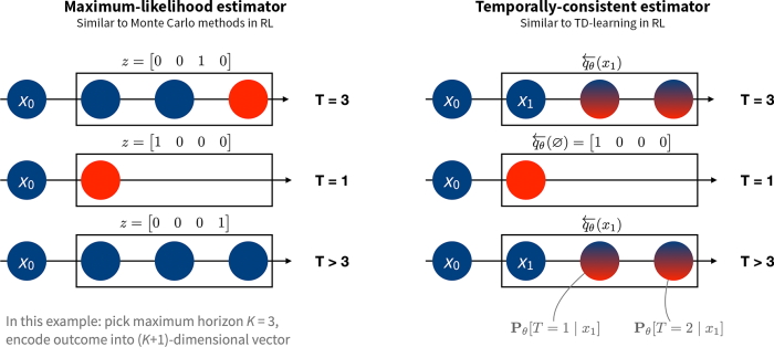
Building on this insight, we develop algorithms that mirror temporal-difference learning, but in the context of estimating a survival model. Instead of using the observed time-to-event (or time to censoring) as the target, we construct a “pseudo-target” that combines the one-hop outcome (whether the event happens at the next step or not) and a prediction about survival at the next state. This difference is illustrated in the figure below.
Benefits of our algorithm
Our approach can be significantly more data-efficient than maximum-likelihood-style direct regression. That is, our algorithm is able to pick up subtle signals that are predictive of survival even when the size of the dataset is limited. This leads to predictive models that are more accurate, as measured by several performance metrics. We demonstrate these benefits in two ways.
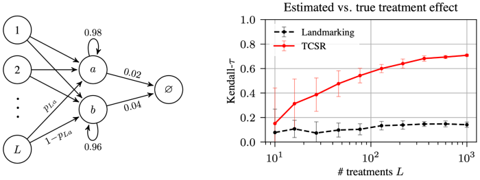
First, we handcraft a task that highlights a setting where our algorithm yields enormous gains. In short, we design a problem where it is much easier to predict survival from an initial state by taking advantage of predictions at intermediate states, as these intermediate states are shared across many sequences (and thus survival from these intermediate states is much easier to learn accurately). We call this the data-pooling benefit, and our approach successfully takes advantage of this. The take-away is that enforcing temporal-consistency reduces the effect of the noise contained in the observed time-to-event outcomes.
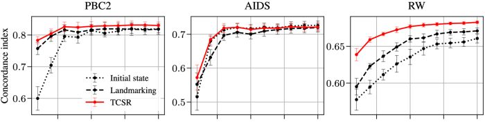
Second, we evaluate models learned using our algorithm empirically on real-world datasets. To facilitate reproducibility, we focus on publicly available clinical datasets, recording survival outcomes of patients diagnosed with an illness. For each patient, biomarkers are recorded at study entry and at regular follow-up visits. In addition, we also consider a synthetic dataset. In each case, we measure a model’s predictive performance as a function of the number of training samples. Models trained using our approach systematically result in better predictions, and the difference is particularly strong when the number of samples is low. In the figure below, we report the concordance index, a popular metric to evaluate survival predictions (higher is better).
A bridge between RL and survival analysis
Our paper focuses mostly on using ideas from temporal-difference learning in RL to improve the estimation of survival models. Beyond this, we also hope to build a bridge between the RL and survival analysis communities. To the survival analysis community, we bring temporal-difference learning, a central idea in RL. Conversely, to the RL community, we bring decades of modeling insights from survival analysis. We think that some RL problems can be naturally expressed in terms of time-to-event (for example, maximizing the length of a session in a recommender system), and we hope that this bridge will be useful. In the paper, we briefly sketch how our approach could be extended to problems with actions, paving the way for RL algorithms tailored to survival settings.
If you are interested in getting hands-on with this, we encourage you to have a look at our companion repository, which contains a reference Python implementation of the algorithms we describe in the paper. For more information, please refer to our paper:
Temporally-Consistent Survival Analysis Lucas Maystre and Daniel Russo NeurIPS 2022
SHARE THIS ARTICLE


