Estimating long-term effects when only short-run experiments are available

Introduction
Quantifying cause and effect relationships is of fundamental importance in many fields, from medicine to economics. The gold standard solution to this problem is to conduct randomised controlled trials, or A/B tests. However, in many situations, such trials cannot be performed; they could be unethical, too expensive, or just technologically infeasible. However, even when randomised controlled trials can be performed, they usually have relatively short durations due to cost considerations. For example, online A/B tests in industry usually last for only a few weeks. This makes learning long-term causal effects a very challenging task in practice, since long-term outcomes are observed only after a long delay. Often short-term outcomes are different to long-term ones, and, as many decision-makers are interested in long-term outcomes, this is a crucial problem to address. For instance, technology companies are interested in understanding the impact of deploying a feature on long-term retention, economists are interested in long-term outcomes of job training programs, and doctors are interested in the long-term impacts of medical interventions, such as treatments for stroke.
In contrast to experimental data, observational data are often easier and cheaper to acquire, so they are more likely to include long-term outcome observations. Previous work by Athey et al. [1] devised a method to estimate long-term causal effects by combining observational long-term data and short-term experimental data. However, this strategy only works if one assumes there are no unobserved confounders in the observational data. This is a strong assumption, as observational data are very susceptible to unmeasured confounding—which can lead to severely biased causal effect estimates.
This leads to the following question: can we combine these short-term experiments with observational data to estimate long-term causal effects when latent confounders are present?
Setting up the problem
We addressed this problem and studied the identification and estimation of long-term causal, or treatment, effects when both short-term experimental data and observational data with latent confounders are available.
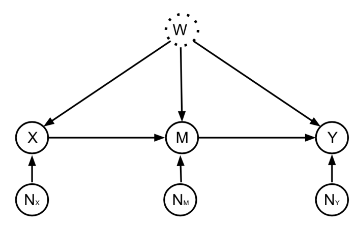
First, to formally state the question posed at the end of the last section, we graphically illustrate the causal structure between our variables of interest in the above directed acyclic graph (DAG). Here, X is the treatment, M is the short-term outcome, and Y is the long-term outcome. We think of M as a mediator between X and Y: the causal impact of X on Y happens indirectly through M. The unobserved confounder is represented as W. The question we aim to solve can now be formally stated:
Given experimental samples between (X, M), and (historical) observational samples between (X, M, Y), can we estimate the causal effect of X on Y?
We initially work with linear structural equation models:
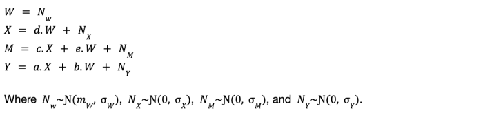
Our long-term causal effect estimator is obtained by combining regression residuals with short-term experimental data in a specific manner to create an instrumental variable, which is then used to quantify the long-term causal effect through instrumental variable regression.
But before we dive into our full solution, let us try a warm up problem to gain some intuition for how we might proceed.
Warm up problem: a new estimator for the front-door causal model
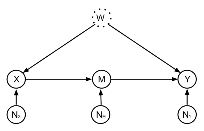
Consider the well-known front-door causal structure, illustrated in the DAG above. Notice the main difference between this DAG and the one from the previous section is that W doesn’t directly cause M in the front-door structure. In the front-door causal structure, to estimate the causal effect of X on Y from observational data, the standard solution is to:
regress M on X to get c,
then regress Y on M and X to get a.
The causal effect is just their product: a.c
Now, instead of the standard estimation strategy outlined above, let’s try something new. Estimating c as before, estimate a as follows:
Regress M on X, and compute the residual: Residual[M|X] = NM
Use NM as an instrumental variable for M -> Y
Given the above DAG, one can see that NM is an instrumental variable for M -> Y because it is independent of W. This realisation is quite powerful, as it allows us to estimate the effect of M on Y. Using NM as an instrumental variable to estimate the effect of M on Y corresponds to regressing Y on NM and M on NM and taking the ratio of the coefficients. This results in a. In the context of the front-door causal structure, this strategy provides a new causal estimator, which may be of independent interest.
We’ll now see that this second strategy to estimating a can be adapted to solve the full problem when W directly causes M.
The full solution
Returning to the first DAG and the full problem, we see that the residual from regressing M on X isn’t the independent noise term NM in this case—due to confounding from W. This means that the residual is correlated with W, and isn't an instrumental variable for M -> Y. However, using the experimental samples between X and M, we can remove the confounding bias on the residual, and use this de-biased residual as an instrument for M -> Y!
That is, in the full problem we can still construct an instrumental variable that can be used to estimate the effect of M on Y in the presence of an unobserved confounder. In our paper, we prove that the following variable

is an instrumental variable for M -> Y. Here, c is the causal effect of X on M obtained from the experimental data, and E(.) is the expectation operator. In our paper, we prove that the instrumental estimator using this variable is unbiased, and analytically study its variance.
We extend this estimator from linear structural causal models to the partially linear structural models routinely studied in economics and prove unbiasedness still holds under mild assumptions. Finally, we empirically test our long-term causal effect estimator, demonstrating accurate estimation of long-term effects on synthetic data, as well as real data from the International Stroke Trial.
Conclusion
Our paper provided a method to combine short-term experiments with long-run observational data to estimate long-term causal effects even when latent confounders are present. Although long-term effect estimation is our primary focus, the estimator and methods described can be applied to any single-stage causal effect. In this context, they can be interpreted as a novel strategy that combines Front-Door and Instrument Variables to estimate causal effects in the presence of unobserved confounders.
For full details, see our paper: Estimating long-term causal effects from short-term experiments and long-term observational data with unobserved confounding Graham Van Goffrier, Lucas Maystre, & Ciarán M. Gilligan-Lee CLeaR (Causal Learning and Reasoning), 2023
References
[1] Athey, Susan, et al. The surrogate index: Combining short-term proxies to estimate long-term treatment effects more rapidly and precisely. No. w26463. National Bureau of Economic Research, 2019.
SHARE THIS ARTICLE

